Entry 1: AprilTag Detection and Pose Estimation

🚀 Starting the Exercise

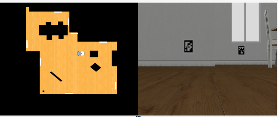
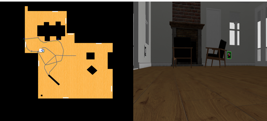
To begin this exercise, I simply displayed the camera capture from the robot to get an initial sense of the setup. When execution starts, the map shows the robot's current position. The front of the robot (where the camera is pointing) is indicated by a small blue triangle, as seen below.

Additionally, the captured image is shown. In this case, two AprilTags are visible — one closer than the other:

🔍 AprilTag Detection

Next, following the exercise guide, I added a function to detect AprilTags in the image using the pyapriltags library, specifying the “tag36h11” family as indicated.

The detector returns a list of detected tags in the image, each with the following information:

• tag_family: The tag family. In this case, "tag36h11".
• tag_id: An integer representing the unique identifier of the tag within its family.
• tag_size: The real-world size of the AprilTag. This is returned as None because no size was specified in the detector. According to the guide: "The AprilTags are set at 0.8 meters in height and have a size of 0.3 x 0.3 meters (the black part is 0.24 x 0.24 meters)."
• hamming: The number of differing bits between the detected tag and the expected code. It is zero.
• decision_margin: A value representing the confidence of the detection.
• homography: A 3x3 matrix representing the projective transformation from the tag’s coordinate system to the image.
• center: A tuple of two values (x, y) representing the center of the tag in pixel coordinates within the image.
• corners: A list of four (x, y) points representing the corners of the detected tag, in the following order:
  • Top-left corner
  • Top-right corner
  • Bottom-right corner
  • Bottom-left corner
• pose_R: A 3x3 rotation matrix representing the orientation of the tag in 3D space.
• pose_t: A 3x1 translation vector representing the position of the tag relative to the camera.
• pose_err: The error associated with the pose estimation.

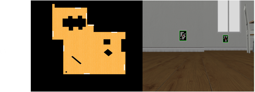
By drawing the lines between the corners and highlighting the tag center, the result is visualized as follows:

🔄 Tag Detection at Various Angles

The initial image is taken with the camera directly facing the tags, but I wanted to test how well the system performs under different conditions.

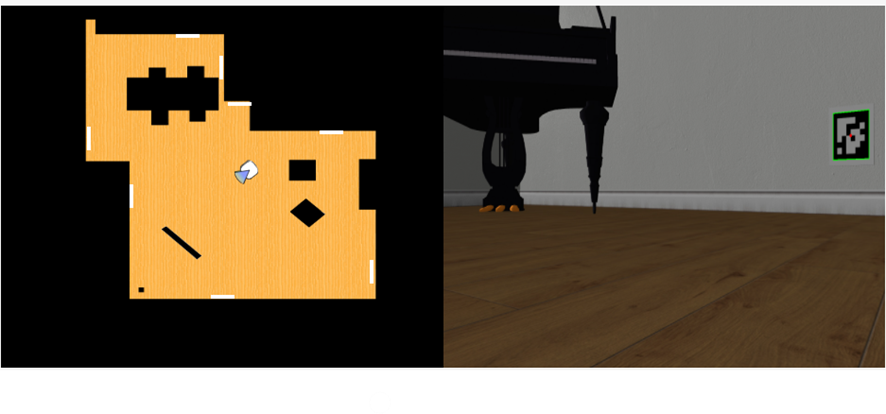
After taking a short random walk around the environment, I observed that even when the AprilTag doesn’t appear as a perfect square, it is still correctly detected. Below are some images that illustrate this:

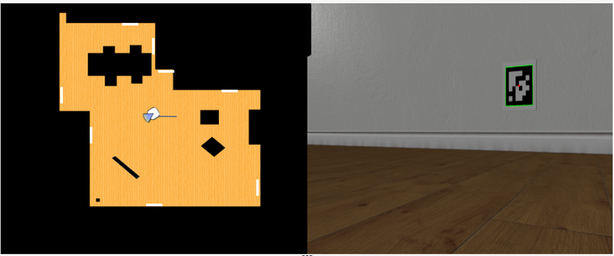
In the next image, two tags appear: one far away, which is successfully detected, and another on the left side, which appears nearly as a thin line due to its extreme angle — and, as expected, is not detected correctly:

Additionally, when the AprilTag is partially occluded (roughly when half of it is out of view), detection fails. This can be clearly seen in the video below: the tag is detected until it exits the right side of the frame.

📍 Getting the Tag's Coordinates

Before estimating the robot’s pose relative to the tag, I visualized the available 3D coordinates of the tag's center along with its 2D image position. Using the provided YAML data and the detected tag IDs, I retrieved their 3D coordinates in the simulated world.

I created a helper function to visualize both 2D and 3D coordinates for debugging:

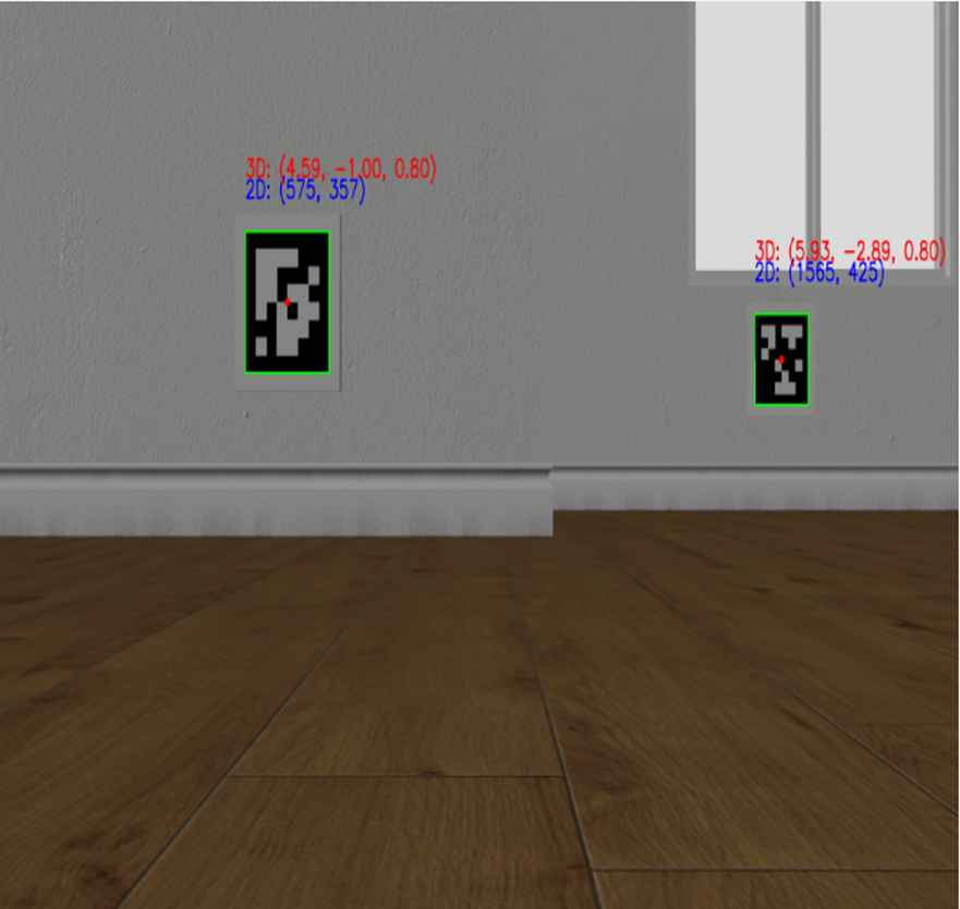
The 3D coordinates refer to the center of the tag in the simulated environment, while the 2D coordinates are from the image. These values will be useful later when transforming the robot’s pose to world coordinates using solvePnP.

📐 SolvePnP

Leaving the previous section aside, the next logical step after detecting the AprilTag is to estimate the robot’s pose with respect to the tag’s reference frame.

That is precisely what I address here. As mentioned, the pose estimation is performed relative to the AprilTag’s coordinate system, where the center is considered to be at (0, 0), and the corners are calculated based on this origin and the tag’s size (as provided in the exercise instructions, 0.3 × 0.3 m total, 0.24 × 0.24 m black region).

Additionally, the corner coordinates detected by the AprilTag detector are needed, along with the camera intrinsic matrix, which is obtained as described in the guide.

With all of this information, I can now apply the solvePnP function, which returns:

• tvec: Camera position relative to the tag
• rvec: Rotation vector (Rodrigues format) relative to the tag

In the video I show below you can see that the operation is performed properly whenever a tag is detected, having some variations with respect to the same tag when the robot changes position, but remaining very similar between iterations. On the other hand, you can see the captured image, in this case showing two apriltags, one closer than the other:

⬅ Back to Exercise 3